Chapter 9: IVEware and SAS

 

9.1 Introduction

Chapter 9 presents examples of common imputation and analytic tasks such as multiple imputation of missing data using IMPUTE, use of BBDESIGN to create a complex sample population data set, descriptive analysis of imputed data using DESCRIBE, linear regression analysis with REGRESS, use of SASMOD (with SAS only) for categorical modeling, use of SYNTHESIZE to create data sets that limit statistical disclosure, and use of COMBINE to combine data from multiple sources.

All examples are run using the SRCShell editor with SAS method, that is, with code submitted from an XML editor and enclosed with <sas> and </sas< tags to run IVEware from within SAS.

National Comorbidity Survey-Replication data is used in many examples. The NCS-R data is derived from a complex sample survey and thus, each example also demonstrates how to correctly account for the design features. For more information on this data set, see the National Comorbidity Survey (NCS) website.

Other data sets used include NHANES 2011-2012 data, Health and Retirement Survey data from 2006, 2008, 2010, and 2012, and Primary Cardiac Arrest data. For information on data sets used in this chapter, see Raghunathan, Berglund and Solenberger (2018) or project specific sites.

Each example includes a short description of the purpose of the example, and the code used. The execution method used in these examples can be easily modified for use with other software such as Stata, R, and SPSS (see Chapter 10 for selected examples of this approach).

Back to top

9.2 IMPUTE Examples

This example uses NCS R data and begins with use of SAS PROC MI with the NIMPUTE=0 option to produce a missing data pattern grid. The grid allows easy visualization of the missing data pattern, amount of missing data per variable and group means for each group in the data set. This command calls on SAS directly and is not part of IVEware.

The second part of the example demonstrates use of IMPUTE and PUTDATA commands to first impute missing data and create M=5 multiples or complete data sets. These imputed data sets are then extracted from a concatenated MI data set using PUTDATA and are available for subsequent analysis.

The 5 imputed data sets extracted are then used as inputs for a number of descriptive and regression analyses to come in later parts of this chapter. In those later examples, we will be analyzing the imputed data sets and using IVEware built-in combining rules appropriate for analysis of multiply imputed data sets as well correct variance estimation for complex sample data.

Syntax:

<sas name=”Impute Example”>
libname d 'P:\IVEware 0.3 documentation 2016\SAS XML Examples';

/* check missing data pattern using SAS PROC MI */
title “Missing Data Pattern from SAS PROC MI” ;
proc mi data=d.ncsr_ex1 nimpute=0 ;
run ;

/* Multiple Imputation using %impute */
<impute name=”MI Using IVEware”>
title Multiple Imputation Using %impute ;
datain d.ncsr_ex1 ;
dataout d.impute_mult1;
default categorical;
continuous bmi intwage ncsrwtsh sestrat ;
transfer caseid ;
iterations 5;
multiples 5;
seed 2001;
run;
</impute>

/* Extract remaining 4 data sets */

<putdata name=”MI Using IVEware” mult=”2″ dataout=”d.impute_mult2″ />
<putdata name=”MI Using IVEware” mult=”3″ dataout=”d.impute_mult3″ />
<putdata name=”MI Using IVEware” mult=”4″ dataout=”d.impute_mult4″ />
<putdata name=”MI Using IVEware” mult=”5″ dataout=”d.impute_mult5″ />

</sas>

 

Selected Output

Multiple Imputation Using %impute

Imputation 1

Variable	Observed	Imputed	Double counted
DSM_GAD	9282	0	0
REGION	9282	0	0
MAR3CAT	9282	0	0
ED4CAT	9282	0	0
NCSRWTSH	9282	0	0
SEX	9282	0	0
SESTRAT	9282	0	0
SECLUSTR	9282	0	0
bmi	8285	997	0
mde	9112	170	0
sexf	9282	0	0
sexm	9282	0	0
ald	9282	0	0
racecat	9282	0	0
ag4cat	9282	0	0
intwage	9282	0	0

 

Back to top

9.2.1 IMPUTE Example with ABB Option

This example uses the ABB option with the IMPUTE command, with the PCA data set. This option permits use of an Approximate Bayesian Bootstrap approach for the imputation model/variable called REDTOT, representing red blood cell total counts.

/* Impute Example with ABB using PCA and Omega 3 Fatty Acids Data */
<sas name=”IMPUTE with ABB Example”>

/* Set libnames */
libname d1 'P:\IVEware_and_MI_Applications_Book\DataSets\PCA and Omega 3 Fatty Acids Data' ;
libname dout 'P:\IVEware 0.3 documentation 2016\SAS XML Examples';

<impute name=”Impute with ABB Option Using PCA and Omega3 Data”>
datain d1.test;
continuous AGE NUMCIG YRSSMOKE FATINDEX DHA_EPA REDTOT WGTKG TOTLKCAL HGTCM ;
categorical CASECNT GENDER RACE3 HYPER DIAB SMOKE FAMMI EDUSUBJ3 CHOLESTH ;
mixed CAFFTOT ALCOHOL3 ;
transfer STUDYID ;
/* Declare ABB for REDTOT, assume non-normal residuals */
ABB redtot ;
restrict NUMCIG(smoke=2,3) YRSSMOKE(smoke=2,3) ;
bounds NUMCIG(>0) YRSSMOKE(>0, <age-12) DHA_EPA(>0) REDTOT(>0) CAFFTOT(>0) TOTLKCAL(>0) ALCOHOL3(>0);
ITERATIONS 3;
MULTIPLES 5;
SEED 2001;
DATAOUT dout.impute_ABB all ;
run;
</impute>

/* Examine Output Data Set*/
proc means data=dout.impute_ABB ;
class _mult_ ;
var redtot ;
run ;

</sas>

 

Back to top

9.2.2 IMPUTE Example with GH Option

Section 9.2.2 demonstrates use of the GH (Tukey's GH) option for the imputation model/REDTOT variable, again using the PCA data set. Like the ABB method, this method can be used to address situations where linear regression is not appropriate.

/* Impute Example with GH using PCA and Omega 3 Fatty Acids Data */
&60;sas name=”IMPUTE with GH Example”>

/* Set libnames */
libname d1 'P:\IVEware_and_MI_Applications_Book\DataSets\PCA and Omega 3 Fatty Acids Data' ;
libname dout 'P:\IVEware 0.3 documentation 2016\SAS XML Examples';

<impute name=”Impute with GH Option Using PCA and Omega3 Data”>
datain d1.test;
continuous AGE NUMCIG YRSSMOKE FATINDEX DHA_EPA REDTOT WGTKG TOTLKCAL HGTCM ;
categorical CASECNT GENDER RACE3 HYPER DIAB SMOKE FAMMI EDUSUBJ3 CHOLESTH ;
mixed CAFFTOT ALCOHOL3 ;
GH redtot ;
transfer STUDYID ;
restrict NUMCIG(smoke=2,3) YRSSMOKE(smoke=2,3) ;
bounds NUMCIG(>0) YRSSMOKE(>0, <age-12) DHA_EPA(>0) REDTOT(>0) CAFFTOT(>0) TOTLKCAL(>0) ALCOHOL3(>0);
ITERATIONS 3;
MULTIPLES 5;
SEED 2001;
DATAOUT dout.impute_gh all ;
run;
</impute>

/* Examine Output Data Set*/
proc means data=dout.impute_gh ;
class _mult_ ;
var redtot ;
run ;
</sas>

 

Back to top

9.3 BBDESIGN Examples

Section 9.3 uses NHANES 2011-2012 adult data to demonstrate examples of the BBDESIGN command.

<sas name=”BBDesign Example”>

/* BBDesign Example, Uses NHANES 2011-2012 DATA with BBdesign and Impute */
libname d 'P:\IVEware_and_MI_Applications_Book\Chapter12Simulations
\Examples\Revised BBDESIGN 12feb2018';

* gather NHANES data where age >=18 and MEC weight > 0
(participated in MEC examination) ;
data nhanes1112_sub_20jan2017 ;
set d.nhanes1112_sub_4nov2015 ;
if age >=18 and wtmec2yr > 0 ;
drop marcat bpxsy1 – bpxsy4 bp_cat pre_hibp bpxdi1 – bpxdi4
dmdmartl irregular ;
run;

proc means nolabels n nmiss mean min max ;
weight wtmec2yr ;
run ;

/* Use BBDesign command to prepare data set using complex
sample design variables and MEC weight:
25 implicate data sets are generated:
5 Bootstrap sample of clusters
5 FPBB using Weighted Polya posterior within each
bootstrap sample
*/

<bbdesign name=”BBdesign”>
datain nhanes1112_sub_20jan2017 ;
dataout d.bbdesignout ;
stratum sdmvstra ;
cluster sdmvpsu ;
weight wtmec2yr ;
csamples 5 ;
wsamples 5 ;
seed 2001;
run;
</bbdesign>

/* Confirm that there are 10 (sample inflation factor)*5,615
(original n) *25 (implicates)= 1,403,750 */
proc freq data=d.bbdesignout ;
tables _impl_ ;
run ;

 

Next, missing data is addressed via use of the IMPUTE command with M=5. Since the data set has already been prepared to represent the population of interest, we impute missing data values for total cholesterol, family income/poverty ratio, BMI, and education within each implicate. Once this is complete, data analysis can be done using simple random sample assumptions, that is, without use of complex sample design variables or probability weights.

/* impute missing data within each of 25 implicates using M=5 and 5 iterations */
<impute name=”Impute_BBDesign”> ;
datain d.bbdesignout ;
dataout d.imputed_samples all ;
default continuous ;
transfer ridstatr seqn ag1829 ag3044 ag4559 ag60 mex
othhis white black other _impl_ _obs_ ;
categorical riagendr ridreth1 edcat ;
bounds indfmpir >= 0, <=5) bmxbmi (>=13, <=80)
lbxtc (>=59, <=523) ;
by _impl_;
seed 2016 ;
multiples 5;
iterations 5;
run ;
</impute> ;

 

Two analyses are now demonstrated; one using a linear regression model and another using logistic regression with combining for both models. This is needed because the default combining rules implemented in REGRESS and PROC MIANALYZE are different from the FPBB rules, see Raghunathan (2016) or Zhou, Elliot and Raghunathan (2016b) for details. The linear regression example uses total cholesterol predicted by gender, BMI, and the ratio of family income to poverty thresholds. For the logistic regression example, a binary outcome of obesity status (coded 1 if BMI >=30, and 0 otherwise) is predicted by age, gender and the income/poverty ratio.

/* Prepare the imputed synthetic populations for analysis */
data synthpops;
set d.imputed_samples;
/*
Create 3 indices S, B, L using the fact that wsamples=5 in
the BBDESIGN code above and given the relationships:
****************************************
indexL=_mult_;
indexS=floor((_impl_-1)/wsamples)+1;
indexB=_impl_-(indexS-1)*wsamples;
****************************************
*/

indexL=_mult_;
indexS=floor((_impl_-1)/5)+1;
indexB=_impl_-(indexS-1)*5;
run ;

/* Save imputed data */
data d.imputed_synthpops
set synthpops ;
male=(riagendr=1) ;
run ;

proc sort data=d.imputed_synthpops;
by indexS indexB indexL;
run ;

/* Estimate of the population mean of lbxtc and its
variance involves 2 steps:
Step 1: Average over IndexB and IndexL for each level
of IndexS */

proc means data=d.imputed_synthpops noprint mean;
var lbxtc;
by indexS;
output out=step1 mean=lbxtcbar;
run ;

/* Step 2: Compute the mean and variance across the
S synthetic populations *

proc means data=step1 mean var ;
var lbxtcbar;
run ;

/* Linear Regression analysis using PROC REG with
imputed synthetic populations*/
proc reg data=d.imputed_synthpops;
by indexS indexB indexL;
model lbxtc = bmxbmi male indfmpir ;
ods output parameterestimates=outparms ;
run ;

title “Print Out from Linear Regression” ;
proc print data=outparms ;
run ;

/* prepare combined estimates and variance using
two data steps*/
proc means data=outparms mean ;
var estimate ;
where variable ='Intercept' ;
by indexs ;
output out=step1_0 mean=bobar ;
run ;

proc print data=step1_0 ;
run ;

proc means data=outparms mean ;
var estimate ;
where variable ='BMXBMI' ;
by indexs ;
output out=step1_1 mean=b1bar ;
run ;

proc print data=step1_1 ;
run ;

proc means data=outparms mean ;
var estimate ;
where variable ='male' ;
by indexs ;
output out=step1_2 mean=b2bar ;
run ;
proc print data=step1_2 ;
run ;

proc means data=outparms mean ;
var estimate ;
where variable ='INDFMPIR' ;
by indexs ;
output out=step1_3 mean=b3bar ;
run ;

proc print data=step1_3 ;
run ;

* Merge temp data sets into 1 for combining ;
data step1_all ;
merge step1_0 step1_1 step1_2 step1_3 ;
by indexs ;
run ;

proc print data=step1_all ;
run ;

* use merged data above for final step ;
proc means data=step1_all mean var noprint;
var bobar b1bar b2bar b3bar;
output out=step2 mean=intercept bmxbmi male indfmpir
var=vintercept vbmxbmi vmale vindfmpir;
run ;

proc print data=step2 ;
run ;

/* Combine results for parameter estimates from above */
data combine_linear ;
set step2;

df=5-1 ; *Min(S-1,C-H);
tvalue=quantile('T',0.975,df);

/* Create arrays for estimate variance se and
lower/upper CI */
array estimate[4] intercept bmxbmi male indfmpir;
array variance[4] vintercept vbmxbmi vmale vindfmpir;
array se[4] se_intercept se_bmxbmi se_male se_indfmpir;
array lower95[4] l95_intercept l95_bmxbmi
l95_male l95_indfmpir;
array upper95[4] u95_intercept u95_bmxbmi
u95_male u95_indfmpir;
do i=1 to 4;
se[i]=sqrt((1+1/5)*variance[i]); * Note that
denominator must match the number used for
“csamples” in the code ;
lower95[i]=estimate[i]-tvalue*se[i];
upper95[i]=estimate[i]+tvalue*se[i];
end;
drop i;
run ;

options nodate nonumber ;
proc print data=combine_linear ;
title “Combined Estimates, SE, Lower and Upper CI from
Linear Regression” ;
var intercept se_intercept l95_intercept
u95_intercept
bmxbmi se_bmxbmi l95_bmxbmi u95_bmxbmi
male se_male l95_male u95_male indfmpir se_indfmpir
l95_indfmpir u95_indfmpir
;
run ;

**********************************************************;

/* Logistic Regression analysis using PROC LOGISTIC,
outcome is obese predicted by male, family income to poverty
and age categories*/

data imputed_synthpops2 ;
set d.imputed_synthpops ;
if bmxbmi >=30 then obese = 1 ; else obese=0 ;
run ;

/*predict probability of being obese by gender and age in
categories and family income to poverty ratio */
proc logistic data=imputed_synthpops2;
by indexS indexB indexL;
model obese (event='1') = male indfmpir ag3044 ag4559 ag60 ;
ods output parameterestimates=outparms_log ;
run ;

proc print data=outparms_log ;
run ;

/* prepare combined estimates and variance using
two data steps*/
/* Create separate mean by IndexS for each variable */

proc means data=outparms_log mean ;
var estimate ;
where variable ='Intercept' ;
by indexs ;
output out=step1_0 mean=bobar ;
run ;

proc print data=step1_0 ;
run ;

proc means data=outparms_log mean ;
var estimate ;
where variable ='male' ;
by indexs ;
output out=step1_1 mean=b1bar ;
run ;

proc print data=step1_1 ;
run ;

proc means data=outparms_log mean ;
var estimate ;
where variable ='INDFMPIR' ;
by indexs ;
output out=step1_2 mean=b2bar ;
run ;

proc print data=step1_2 ;
run ;

proc means data=outparms_log mean ;
var estimate ;
where variable ='ag3044' ;
by indexs ;
output out=step1_3 mean=b3bar ;
run ;

proc print data=step1_3 ;
run ;

proc means data=outparms_log mean ;
var estimate ;
where variable ='ag4559' ;
by indexs ;
output out=step1_4 mean=b4bar ;
run ;

proc print data=step1_4 ;
run ;

proc means data=outparms_log mean ;
var estimate ;
where variable ='ag60' ;
by indexs ;
output out=step1_5 mean=b5bar ;
run ;

proc print data=step1_5 ;
run ;

data step1_all_log ;
merge step1_0 step1_1 step1_2 step1_3 step1_4 step1_5;
by indexs ;
run ;

proc print data=step1_all_log ;
run ;

/* Prepare combined estimates and variance
using two data steps*/
proc means data=step1_all_log mean var ;
var bobar b1bar b2bar b3bar b4bar b5bar;
output out=step2_log mean=intercept male indfmpir
ag3044 ag4559 ag60
var=vintercept vmale vindfmpir vag3044 vag4559 vag60;
run ;

/* Combine results for logistic regression */
data combine_log ;
set step2_log ;
df=5-1 ; *Min(S-1,C-H);
tvalue=quantile('T',0.975,df);

/* Create arrays to the calculations */
array estimate[6] intercept male indfmpir ag3044
ag4559 ag60;
array variance[6] vintercept vmale vindfmpir vag3044
vag4559 vag60;
array se[6] se_intercept se_male se_indfmpir
se_ag3044 se_ag4559 se_ag60 ;
array lower95[6] l95_intercept l95_male l95_indfmpir
l95_ag3044 l95_ag4559 l95_ag60;
array upper95[6] u95_intercept u95_male u95_indfmpir
u95_ag3044 u95_ag4559 u95_ag60;
array or[6] or_intercept or_male or_indfmpir
or_ag3044 or_ag4559 or_ag60;
do i=1 to 6;
se[i]=sqrt((1+1/5)*variance[i]);
or[i]=exp(estimate[i]);
lower95[i]=exp(estimate[i]-tvalue*se[i]);
upper95[i]=exp(estimate[i]+tvalue*se[i]);
end;
drop i;
run ;

proc print data=combine_log ;
title “Combined Estimates from Logistic Regression” ;
run ;

</sas>

 

Back to top

9.4 DESCRIBE Example

The DESCRIBE example, using NCS-R data, presents a descriptive analysis of age at interview and body mass index with a gender contrast. The example uses the 5 imputed data sets from IMPUTE along with MI combining rules and design-based variance estimation using the default TSL method. Use of the STRATUM, CLUSTER, and WEIGHT statements declare the complex sample design variables and weight to the software. The CONTRAST statement requests a linear contrast of mean age at interview and Body Mass Index by gender. The DESCRIBE command with a mean statement produces a means analysis of age at interview and BMI. Missing data is excluded, resulting in a complete case analysis.

<sas name=”DESCRIBE Example using Imputed Data Sets”>
libname d “P:\IVEware 0.3 documentation 2016\SAS XML Examples”;

/* Descriptive Analysis of Age at Interview and BMI, Missing Data Imputed by IVEware */
<describe name=”DESCRIBE Example Using Imputed
Data Sets with Design Adjusted Imputed Descriptive Analysis of Age and BMI”>
title MI Design-based Description;
datain d.impute_mult1 d.impute_mult2 d.impute_mult3 d.impute_mult4 d.impute_mult5 ;
stratum sestrat;
cluster seclustr;
weight ncsrwtsh ;
model mult;
mean intwage bmi;
contrast sexf;
run;
</describe>
</sas>

 

Back to top

9.5 REGRESS Example

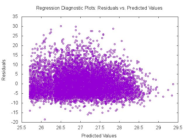
The REGRESS example again uses the previously imputed NCS-R data sets as inputs. This example regresses body mass index (BMI) on lifetime Major Depressive Episode, an indicator of being female, and age at interview. The default variance estimation method in REGRESS is the Jackknife Repeated Replication method. Use of the PLOTS statement will produce a number of diagnostic plots with a .png extension. Note that the gnuplot software must be included in the 'settings' file (stored in the SRCLIB folder where software installed) for this to work correctly. One diagnostic plot is included in the selected output given below.

<sas name=”REGRESS Example using Imputed Data Sets”>
libname d “P:\IVEware 0.3 documentation 2016\SAS XML Examples”;

/* Analyze Five Previously Imputed Data Sets using Linear Regression with REGRESS*/
/* Example uses Complex Sample Design Variables and Diagnostic Plots */

<regress name=”Linear Regression Example”>
title Linear Regression using REGRESS with Imputed Data Sets;
datain d.impute_mult1 d.impute_mult2 d.impute_mult3 d.impute_mult4 d.impute_mult5 ;
estout impute_regress;
stratum sestrat;
cluster seclustr;
weight ncsrwtsh;
dependent bmi;
predictor mde sexf intwage ;
link linear ;
plots outplots ;
run;
</regress>
</sas>

 

Selected Regression Output

All imputations
Valid cases	9282
Sum weights	9282.000152
Degr freedom	26.42925062
Sum of squares:
Model	3954.942524
Error	299501.0663
Total	303456.0088
R-square	0.01303
F-value	0.08725
P-value	0.98565

Variable	Estimate	Std Error	T Test	Prob > |T|
Intercept	25.9222187	0.2549001	101.69559	0.00000
mde	0.8287332	0.1234398	6.71366	0.00000
sexf	-0.6898597	0.1395496	-4.94347	0.00004
intwage	0.0290391	0.0049550	5.86059	0.00000

Variable	Estimate	95% Confidence Interval
		Lower	Upper
Intercept	25.9222187	25.3986774	26.4457600
mde	0.8287332	0.5751993	1.0822672
sexf	-0.6898597	-0.9764816	-0.4032378
intwage	0.0290391	0.0188620	0.0392162

Variable	Design Effect	SRS Estimate	% Diff SRS v Est
Intercept	1.48293	26.3002986	1.45852
mde	0.60113	0.8344926	0.69496
sexf	1.17056	-0.6735030	-2.37102
intwage	1.58580	0.0231927	-20.13297

Back to top

9.6 SASMOD Example

The SASMOD command is available with IVEware and SAS only. This command is based upon the Jackknife Repeated Replication method for variance estimation and can be used with many SAS procedures (see previous sections of this chapter). In this example, PROC CATMOD is used to execute an MI and design-based log-linear model. The model examines relationships between gender and Major Depressive Episode, using the 5 previously imputed NCS-R data sets as input.

<sas name=”SASMOD with PROC CATMOD”>

libname d 'P:\IVEware 0.3 documentation 2016\SAS XML Examples';

/* Analyze 5 Imputed Data Sets with JRR Variance Estimation PROC CATMOD for Log-Linear Model */
<sasmod name=”SASMOD for Log-Linear Model with PROC CATMOD”>
title SASMOD Example ;
datain d.impute_mult1 d.impute_mult2 d.impute_mult3 d.impute_mult4 d.impute_mult5 ;
estout modexam;
cluster seclustr ;
stratum sestrat ;
weight ncsrwtsh;

/* SAS statements begin here */
proc catmod;
model mde*sexf =_response_ / pred=freq;
loglin mde sexf mde*sexf ;
run;
</sasmod>
</sas>

Selected Output

All imputations
Valid cases	9282
Sum weights	9282.000152
Degr freedom	Infinite
-2 LogLike	21833.80757

Variable	Estimate	Std Error	Wald test	Prob > Chi
mde 0	0.7346635	0.0173232	1798.53648	0.00000
sexf 0	-0.1223741	0.0115333	112.58311	0.00000
mde*sexf 0 0	0.1283257	0.0168590	57.93785	0.00000

Variable	Estimate	95% Confidence Interval
		Lower	Upper
mde 0	0.7346635	0.7006693	0.7686577
sexf 0	-0.1223741	-0.1450064	-0.0997418
mde*sexf 0 0	0.1283257	0.0952424	0.1614090

 

Back to top

9.7 SYNTHESIZE Examples

9.7.1 Fully Synthesized Data Set

The first SYNTHESIZE example demonstrates multiple imputation of missing data followed by synthesis of each variable in the Primary Cardiac Arrest data set. In the code below, we request 5 multiple imputations with 5 implicates or synthesized data sets per imputation multiple. Use of similar syntax as from IMPUTE is utilized along with the SYNTHESIZE statement to declare the variables to be synthesized. The imputation is done before the synthesis, therefore each of 5 imputation multiples contains 5 synthesized data sets for subsequent analysis. Two key variables are created during this process: IMPL with values of 1,2,3,4,5 denoting synthesized data sets 1-5, and MULT with values of 1,2,3,4,5 denoting imputations. The final part of this example demonstrates correct combining rules for fully synthesized and imputed data (Raghunathan (2015), page 168).

/* Synthesize Example Using PCA and Omega 3 Fatty Acids Data */
<sas name=”SYNTHESIZE Example”>
/* Set libnames */
libname d1 'P:\IVEware_and_MI_Applications_Book\DataSets\PCA and Omega 3 Fatty Acids Data' ;
libname dout 'P:\IVEware 0.3 documentation 2016\SAS XML Examples';

<synthesize name=”Synthesize All Variables Using PCA and Omega3 Data”>
datain d1.test;
continuous AGE NUMCIG YRSSMOKE FATINDEX DHA_EPA REDTOT WGTKG TOTLKCAL HGTCM ;
categorical CASECNT GENDER RACE3 HYPER DIAB SMOKE FAMMI EDUSUBJ3 CHOLESTH ;
mixed CAFFTOT ALCOHOL3 ;
transfer STUDYID ;
synthesize CASECNT AGE GENDER RACE3 HYPER DIAB SMOKE NUMCIG YRSSMOKE FATINDEX
FAMMI EDUSUBJ3 DHA_EPA REDTOT CHOLESTH CAFFTOT WGTKG TOTLKCAL ALCOHOL3 HGTCM ;
restrict NUMCIG(smoke=2,3) YRSSMOKE(smoke=2,3) ;
bounds NUMCIG(>0) YRSSMOKE(>0, <age-12) DHA_EPA(>0) REDTOT(>0)
CAFFTOT(>0) TOTLKCAL(>0) ALCOHOL3(>0);
ITERATIONS 2;
MULTIPLES 5;
SEED 2001;
IMPLICATES 5;
DATAOUT dout.synthesize all ;
run;
</synthesize>

/* Examine Contents of Output Data Set*/
proc contents data=dout.synthesize ;
run ;

data synthesized ;
set dout.synthesize ;
* use implicates 1-5 only ;
if _impl_ >=1 then _imputation_= cat(_mult_, _impl_) ;
run ;

proc freq ;
tables _mult_*_impl_ _imputation_ ;
run ;

proc sort data=synthesized ;
by _imputation_ ;
run ;

/* Obtain mean kcalories per day by _imputation_ and then combine using correct rules for synthesized data*/
proc means data=synthesized (where=(_imputation_ ne ' ' )) mean stderr ;
var totlkcal ;
by _imputation_ ;
ods output summary=outstat ;
run ;
proc print data=outstat ;
run ;

proc sql ;
create table outstat1
as select *, mean(totlkcal_mean) as qbar, mean(totlkcal_stderr*totlkcal_stderr) as ubar
from outstat ;
proc sql ;
create table outstat2
as select *, sum((totlkcal_mean – qbar)**2)/24 as btwvar
from outstat1

/* Combining rules for fully imputed and synthesized data*/
data final ;
set outstat2 ;
if _n_=1 ;
syn_estimate=qbar ;

syn_variance=ubar ;
syn_se=sqrt(syn_variance) ;
btw=btwvar ;
total_syn_var=((1+1/25)*btwvar) – ubar ;

proc print data=final ;
var syn_estimate syn_se syn_variance btwvar total_syn_var;
run ;

 

Results from Fully Synthesized Data Set

Parameter	Mean	SE	Total Variance
Total Kilocalories	1822.24	40.44	106.10

Back to top

9.8 COMBINE Example

The COMBINE example joins four waves of Health and Retirement Survey data from 2006, 2008, 2010 and 2012. Though the data sets have the same variable names and values, each has manufactured missing data on some variables. For example, the HRS 2006 data has no observed data on three variables: DIABETES, ARTHRITIS, and SELFRHEALTH, HRS 2008 data is completely missing on DIABETES and ARTHRITIS but has observed data on SELFRHEALTH, and so on. In addition, other variables such as marital status (MARCAT) have small amounts of missing data in some or all waves of data. This example demonstrates a three step process: 1. 'stacking' the data using COMBINE, 2. imputing the missing data in the combined data set using IMPUTE, and 3. use of DESCRIBE to perform MI and design-based descriptive analysis of arthritis by year.

<sas name=”COMBINE Example using 4 Waves of HRS Data”>
libname d “P:\IVEware_and_MI_Applications_Book\Chapter2DataSources”;

/* COMBINE Example Using HRS 2006 2008 2010 and 2012 Data */
<combine name=”COMBINE Example”>
datain d.hrs2006_27jul2016 d.hrs2008_27jul2016 d.hrs2010_27jul2016 d.hrs2012_27jul2016 ;
dataout d.combined_hrs_2006_2012 ;
run;
</combine>

/* Use SAS to Examine Contents of Combined Data */
proc contents data=d.combined_hrs_2006_2012 ;
run ;

/* Examine Means of Combined Data */
proc means n nmiss mean min max data=d.combined_hrs_2006_2012 ;
class yr ;
run ;

/* Use IMPUTE to impute missing data */
<impute name=”Impute_Post_COMBINE”>
datain d.combined_hrs_2006_2012 ;
dataout d.impute_mult1;
default categorical;
continuous stratum age wgt;
transfer hhid pn ;
iterations 5;
multiples 5;
seed 2016 ;
run;
</impute>

/* Extract remaining 4 data sets */
<putdata name=”Impute_Post_combine” mult=”2″ dataout=”d.impute_mult2″ />
<putdata name=”Impute_Post_combine” mult=”3″ dataout=”d.impute_mult3″ />
<putdata name=”Impute_Post_combine” mult=”4″ dataout=”d.impute_mult4″ />
<putdata name=”Impute_Post_combine” mult=”5″ dataout=”d.impute_mult5″ />

/* Use Imputed Data Sets for Descriptive Analysis*/
<describe name=”Descriptive Analysis of Combined and Imputed Arthritis by Year”>
datain d.impute_mult1 d.impute_mult2 d.impute_mult3 d.impute_mult4 d.impute_mult5 ;
stratum stratum ;
cluster secu;
weight wgt ;
table arthritis ;
by yr ;
run;
</describe>

</sas>

 

Proportion of Arthritis by Year, Based on Combined, Imputed HRS Data

Outcome	Year	Mean	SE
Diagnosis of Arthritis	2006	0.548	0.007
“	2008	0.567	0.008
“	2010	0.532	0.006
“	2012	0.550	0.008

Back to top