We often talk about “data quality” or “data integrity” when we are discussing the collection or analysis of one type of data or another. Yet, the definition of these terms might be unclear, or they may vary across different contexts. In any event, the terms are somewhat abstract — which can make it difficult, in practice, to improve. That is, we need to know what we are describing with those terms, before we can improve them.

Over the last two years, we have been developing a course on Total Data Quality, now available on Coursera. We start from an error classification scheme adopted by survey methodology many years ago. Known as the “Total Survey Error” perspective, it focuses on the classification of errors into measurement and representation dimensions. One goal of our course is to expand this classification scheme from survey data to other types of data.

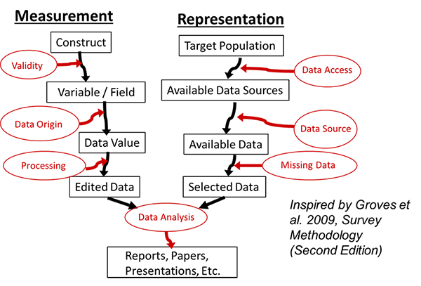
The figure shows the classification scheme as we have modified it to include both survey data and organic forms of data, also known as big data or found data. We find that all forms of data are subject to these same sorts of errors in varying degrees.

We won’t define all the classes in this post – just two examples.

Data Origin

First, on the measurement side, we look at “Data Origin” as how were the individual values / data points for a given variable (or field) recorded, captured, labeled, gathered, computed, or represented? This could be the process of answering a question, filling a field in an administrative record, or labeling an image in a machine learning context. In the case of labeling images, this could be a human being incorrectly labeling an image. For example, a human being might not note the difference between a cat or a kitten. In some contexts, that difference could be important.

Missing Data

On the representation side, “Missing Data” is a common problem that impacts many types of data. For example, administrative records can be missing key variables or even entire records. Similar things can happen with surveys. These missing data can impact inferences or predictions if the missing values differ from the observed values in important ways.

Using this classification scheme as a way to think about errors can help guide researchers as they consider quality issues. Further, being aware of these issues may also open the door to enhancing the quality along these dimensions! If you’d like to learn more, our new open online courses series focuses on identifying, measuring, and maximizing quality along all of these dimensions.

The post was originally published on Survey Methods Musings.

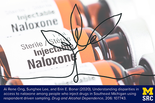
Ai Rene Ong, who is a doctoral candidate in the Michigan Program in Survey Methodology and a research assistant in the Survey Methodology Program (SMP), recently collaborated with SMP faculty member Sunghee Lee and Dr. Erin Bonar from the University of Michigan Addiction Center to publish an original research investigation entitled ‘Understanding disparities in access to naloxone among people who inject drugs in Southeast Michigan using respondent driven sampling‘ in the journal Drug and Alcohol Dependence. Naloxone is a critical, life-saving antidote for people who have overdosed on prescription opioids, which unfortunately is becoming much more common in today’s society, especially among injection drug users. These high-risk populations are also harder to identify, sample, and measure, which is where respondent driven sampling (RDS), a technique that Dr. Lee specializes in, becomes so valuable.

This research team analyzed data collected as part of the project Positive Assessment Towards Health (PATH). In 2017, PATH recruited 46 seeds, who in this case were persons who inject drugs (PWID), to complete self-administered questionnaires and spread the word about this research project among their peers. The seeds, who received a $30 incentive for participating, were recruited from local agencies and community health clinics in Southeastern Michigan serving PWID. Following RDS techniques, the seeds were given three recruitment coupons and asked to recruit their PWID peers. Participants received $10 per successful recruit. PATH ultimately recruited a total of 410 PWID from Southeastern Michigan to participate in the study. The participants completed Audio Computer-Assisted Self-Administered Interviewer (ACASI) questionnaires at community and health centers. The questionnaires collected information on substance use behaviors and access to naloxone, among other related topics. The research team then computed descriptive statistics using weighted estimators appropriate for RDS (using the inverse of the self-reported network size as a weight), and fitted logit models to these data using the same weights, predicting self-reported naloxone access as a function of socio-demographics, health indicators, substance use history, and geographic information.

The authors found evidence of significant disparities in access as a function of geography (where urban individuals were much less likely to have access), race/ethnicity (where non-Hispanic blacks and those of other races/ethnicities had lower odds of having access relative to non-Hispanic whites), socio-economic status (e.g., access was substantially more likely for those with higher income), and recent homelessness (where those recently homeless were much more likely to have access). However, given the study sites (i.e. urban represented by Detroit), the geographical disparities in naloxone access may be due to the sociodemographic characteristics of these locations (i.e., a high proportion of non-Hispanic black PWID in Detroit). In addition, people with a history of prior opioid abuse were significantly more likely to have access. No age or gender differences were identified.

Overall, the results of this study suggest that access to naloxone among PWID, who are at high risk of opioid overdose, appears to be particularly low (an estimated 24.9% of individuals in this population have access), at least in Southeastern Michigan. Future work could certainly explore this issue in other communities to see if the same issues emerge elsewhere, and RDS is a promising technique for collecting these important data from these types of hard-to-reach populations. This work suggests that recent policies designed to increase naloxone access may not be entirely effective, especially for particularly high-risk subgroups, and the fact that RDS was able to shed light on this issue should be leveraged by substance abuse researchers from other communities in the future to better understand this important public health problem.

Ai Rene Ong, Sunghee Lee, and Erin E. Bonar (2020). Understanding disparities in access to naloxone among people who inject drugs in Southeast Michigan using respondent driven sampling. Drug and Alcohol Dependence, 206: 107743.

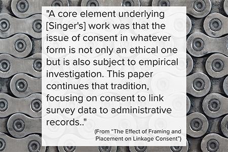
Together with their international colleagues Alexandra Schmucker and Frauke Kreuter, adjunct Survey Methodology Program (SMP) faculty member and Program in Survey Methodology (PSM) graduate Joe Sakshaug, SRC Research Professor Mick Couper, and the late SRC Research Professor Eleanor Singer recently published a research note entitled ‘The Effect of Framing and Placement on Linkage Consent‘ in a special issue of Public Opinion Quarterly. This special issue of POQ honored Eleanor’s long history of excellent research contributions. This specific article by Sakshaug and colleagues emphasizes the importance of strategies for optimizing respondent consent to record linkage so that surveys can maximize the benefits of linking survey responses to external data sources, including administrative records.

The study described in the article featured a randomized experiment evaluating the effects of two critical factors in this process: the way that the question about record linkage is framed (‘gain’ framing, emphasizing the positive aspects of consenting to linkage, and ‘loss’ framing, emphasizing how the survey would be affected by a failure to consent), and where in the survey process the question is asked (at the beginning of the survey, or at the end). Respondents in two separate surveys (a telephone survey, n = 677; and a web survey, n = 651) were randomly assigned to one of four groups defined by the cross-classification of the two levels of each experimental factor.

The authors reported evidence of a significant interaction between the two factors in each survey. In the web survey, a significant positive effect of ‘loss’ framing was only found when the consent question was placed at the end of the questionnaire. In the telephone survey, the effect of ‘loss’ framing actually changed directions depending on placement: this type of framing had a negative effect on the consent rate when the question was placed at the beginning of the survey, and a positive effect when placed at the end of the survey. In both surveys, the placement effect was larger than the framing effect, where placement at the beginning of the survey was found to consistently increase consent rates. Overall, placement was found to be the most important factor, and the authors provided evidence of the importance of placing this question at the beginning of the survey, regardless of the survey mode.

This study was also unique in that the authors had access to administrative data for both individuals consenting to record linkage and individuals not consenting, enabling calculations of consent bias (and not just consent rates) associated with the two factors. The authors report that neither experimental factor affected consent bias in any meaningful way. Survey researchers working on surveys including this type of consent question should feel reassured by these findings.

Overall, this was a well-designed study that provides clear evidence in support of a design feature that survey researchers interested in record linkage can easily manipulate to optimize consent rates. The important and practical take-away points should appeal to survey researchers engaged in survey projects asking respondents to consent to record linkage.

Joseph W Sakshaug, Alexandra Schmucker, Frauke Kreuter, Mick P Couper, and Eleanor Singer (2019). The Effect of Framing and Placement on Linkage Consent. Public Opinion Quarterly, 83(S1): 289-308.

By: Xinyu Zhang

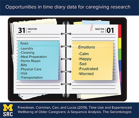
Previous studies have well documented caregivers for older adults’ declined wellbeing. However, most studies use relatively less fine-grained measures that left the role of specific care activities in the daily lives unanswered. In a recent study published in The Gerontologist, SRC researcher Vicki Freedman and her colleagues used time diary data from the 2013 Disability and Use of Time (DUST) supplement to the Panel Study of Income Dynamics (PSID) to explore patterns of informal caregiving and experienced wellbeing over the day.

The measures in most studies of caregiving are not perfect. For example, respondents were typically asked to answer yes/no or to recall the number of hours in a typical week or month. These ways of measuring time spent on caregiving fail to capture precisely how time is spent on each task throughout the day. In addition, decontextualized wellbeing measures (e.g., ask respondents to recall their overall wellbeing over a reference period) cannot specifically evaluate the impact of caregiving.

Comparing to studies using aggregated measures of time use, the detailed diary data can capture both time use on specific tasks and momentary wellbeing. The diary interview asked about all activities happened on the previous day over a 24-hour period. The authors created ordered indicators of care for each 15-min interval. Caregiving activities were categorized as not care, household care, physical care, visiting/socializing, and transportation. To measure experienced wellbeing, respondents were asked to report how intensely they felt five emotions for up to three randomly selected diary activities.

The study found that caregivers on average spent 2.3 hours per day on caregiving, which is an hour less than global reports of care provided on the prior day with the DUST sample. One possible explanation of this result is social desirability effect; social pressure to over-report socially-favored activities relative to diary measure.

The researchers performed sequence and cluster analysis to characterize type and time of care activity. The result showed participation in care follows a roller-coaster pattern over the day, reaching peaks around mealtimes (10 a.m., 12p.m., and 5 p.m.). Five care types were identified with different intensities and activities. The authors found that 40% of caregivers provided only marginal assistance of about 1 hour per day and 28% provided sporadic assistance with a mix of activities for about 2 hours. Interestingly, marginal assistance providers reported lower experienced wellbeing than sporadic assistance providers. Their innovative work portrayed the patterns of older adults’ varying caregiving activities and further explored caregivers’ wellbeing.

Vicki Freedman, Jennifer Cornman, Deborah Carr, and Richard Lucas (2019). Time Use and Experienced Wellbeing of Older Caregivers: A Sequence Analysis. The Gerontologist.

In a paper published recently in the Public Opinion Quarterly, SRC’s Fred Conrad, with lead author Josh Pasek and co-authors Yanna Yan, Frank Newport, and Stephanie Marken, explored the ways that Twitter data are generated to find ways to predict when social media and survey data provide similar information in the area of consumer confidence. An important difference between national surveys and Twitter is that surveys use scientific methods to choose a sample that is representative of the U.S. whereas Twitter may only be representative of Twitter users. That is, does information from Twitter tell us something about national trends or only about trends within the population of Twitter users.

Almost since the advent of social media, scientists have recognized its potential as a source of social information for research. For example, flu epidemics can be followed by tracking mentions of sick, sneeze, and cough on Twitter. An open question is when and how social media and survey information are aligned. This is important because obtaining information from social media is much less expensive than collecting information through surveys. Understanding more about when and how social media information provides a useful complement and potentially a supplement for survey information may pave the way for wider usage in scientific discovery.

To understand this more, these researchers compared data from the Michigan Surveys of Consumers and other data sources with information from Twitter under two conditions:

• A simple comparison of Twitter with national survey data
• A comparison of Twitter with survey data that have been weighted to reflect Twitter users

Following previous research showing that Tweets with the word ‘jobs’ in them tend to track with measures of consumer confidence, the researchers used this same strategy in their present study. They compared survey data to Twitter data over a 5 year period from 2008 to 2013, that is over the period of the Great Recession.

Some of their findings support the idea that under certain conditions, social media information indicative of consumer sentiment does tend to mirror that obtained from surveys. These conditions appear to be highly changeable, however. The alignment of survey data and social media information on consumer confidence is closer under more volatile economic conditions. It may be that Twitter is tapping into public attention to newsworthy changes, such as the dramatic events surrounding the Great Recession. Interestingly, when the researchers adjusted the data to reflect the Twitter using population, the alignment of survey data and Twitter data was no closer. At least for consumer sentiment, Twitter users over this time appeared to be in line with the Nation as a whole.

Pasek, Josh, H. Yanna Yan, Frederick G. Conrad, Frank Newport, Stephanie Marken (2019). The Stability of Economic Correlations over Time: Identifying Conditions under Which Survey Tracking Polls and Twitter Sentiment Yield Similar Conclusions. Public Opinion Quarterly, 82(3): 470-492.

Dr. Jack Kuang Tsung Chen (Program in Survey Methodology PhD 2016), along with SRC researchers Drs. Richard Valliant and Michael Elliott conducted a study that explores and evaluates approaches to combining data from probability and non-probability surveys. Recently published in the Journal of the Royal Statistical Society: Series C (Applied Statistics), and based on Chen’s dissertation, this work used data collected from high-quality probability samples that produce unbiased estimates, but are time-consuming and expensive to collect, to adjust data from non-probability samples that may be tainted by selection bias, but are cheaply and easily obtained.

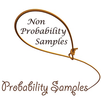
As senior author Dr. Elliott explains, ‘… a major issue implied by this type of work is that probability and non-probability sampling are synergistic rather than antagonistic — the proliferation of administrative and non-probability sample data for social science research means that having a small “corral” of high-quality probability samples is more important than ever to assist with calibration, imputation, and other adjustment methods.’

This article developed and advocated estimated control least angle shrinkage and selection operator (ECLASSO) regression. This approach extends the existing LASSO approach by incorporating sampling-related measurement error in benchmark probability-sample data into the variance component of model-assisted calibration estimators. LASSO is a useful approach to calibration because it automates both variable selection and parameter estimation for the model used to calibrate a given (likely non-probability) sample to control totals from the probability sample using a penalized regression approach to avoid overfitting.

As the authors explain, their approach ‘combines both quasi-likelihood and modelling approaches by utilizing a probability-based benchmark sample … (together with) an assisting model to predict an outcome of interest, given a set of calibration variables that exists in both probability and non-probability samples. The outcome variable in the non-probability sample is then calibrated to the predicted outcome total in the probability sample, given the probability sampling weights in the benchmark data.’ Simple, right?

LASSO can accommodate numerous predictors in the calibration model, even when using a small probability sample for calibration. The authors note that ‘(b)ecause we are relying so heavily in non-probability samples on models that can approximate the expected value of (an outcome variable of interest) to compensate for the lack of design weights, a large number of covariates and, consequently, control totals may be required to obtain accurate models.’ Both the non-probability data source and the benchmark probability sample data must contain the same outcome variable and substantively and empirically related covariates.

ECLASSO, like all such calibration approaches, assumes the full spectrum of values of model variables in the population has non-zero probability of being observed in both analytical and benchmark samples. This places a quality constraint on the non-probability sample, requiring that it must not be so extreme in its under-coverage that some covariate values are unrepresented.

The authors used large non-probability samples from SurveyMonkey with data on voting preferences for US Senate and state gubernatorial candidates in the 2014 midterm elections, along with probability sample data from the same time period collected by the Pew Research Center, to compare the accuracy and efficiency of election outcome estimates using a number of calibration techniques.

They compare ECLASSO to: 1) unweighted estimates from the non-probability data, 2) a weighting-class adjustment using census data, 3) propensity score weighting using the Pew data, and 4) the estimated control generalized regression estimator (ECGREG). Using the election results as the gold standard, when compared to the other calibration techniques, ECLASSO-derived point estimates had the smallest average absolute bias and relative error. This accuracy, paired with standard errors comparable to those obtained via weighting-class adjustment, resulted in ECLASSO having the lowest RMSE and best confidence interval coverage of the five approaches considered.

Chen and his co-authors also conducted a simulation study using the 2013 National Health Interview Survey (NHIS) as the benchmark study, while also using NHIS to simulate internet-based non-probability samples. Again, ECLASSO outperformed naïve (equal probability) treatment of the biased sample data, as well as GREG and propensity score approaches.
The authors demonstrated that contemporary approaches such as ECLASSO, although complex, can provide improvement over standard linear regression and weighting-class approaches to calibration and imputation.

Although there is much promise in using data from non-probability samples, any sound method of doing so may need to rely on data from high quality probability surveys in specific research areas to provide a source of calibration measures for the adjustment of the data from non-probability sources. This suggests that the lights will burn brightly in the SRC sampling section for many years to come.

Chen, Jack Kuang Tsung; Valliant, Richard L.; Elliott, Michael R. (2018). Calibrating non-probability surveys to estimated control totals using LASSO, with an application to political polling. Journal of the Royal Statistical Society: Series C (Applied Statistics).

By: Patricia Berglund

Description of IVEware

IVEware is a collection of routines written under various platforms and packaged to perform multiple imputations, variance estimation and, in general, draw inferences from incomplete data. The software can also be used to perform analysis without any missing data. IVEware defaults to assuming a simple random sample, but uses the Jackknife Repeated Replication or Taylor Series Linearization techniques for analyzing data from complex surveys.

The latest version is 0.3 but previous versions of 0.1 and 0.2 are still available for download from iveware.org. Version 0.1 is a command based tool while 0.2 provides a GUI interface.

Overview of ‘Multiple Imputation in Practice: With Examples Using IVEware’

Multiple Imputation in Practice: With Examples Using IVEware provides practical guidance on multiple imputation analysis, from simple to complex problems using real and simulated data sets. Data sets from cross-sectional, retrospective, prospective and longitudinal studies, randomized clinical trials, complex sample surveys are used to illustrate both simple, and complex analyses.

Version 0.3 of IVEware, the software developed by the University of Michigan, is used to illustrate analyses. IVEware can multiply impute missing values, analyze multiply imputed data sets, incorporate complex sample design features, and be used for other statistical analyses framed as missing data problems. IVEware can be used under Windows, Linux, and Mac, and with software packages like SAS, SPSS, Stata, and R, or as a stand-alone tool.

The data sets for the examples and exercises and the example code files are available to download. The figures, many of which are reproduced in color, are also available.

Order the book at CRC Press or Amazon.

The frequent occurrence of sexual assaults on college campuses has focused national attention on this important public health concern, with estimates of sexual assault rates as high as 20% reported for undergraduate women. However, an important knowledge gap exists regarding rates of sexual assault for young adults in general, in that accurate population-based prevalence rates for both women and men who do and do not attend college are not readily available.

In a recent study, SRC Research Professor William Axinn, SRC Research Associate Professor Brady West, and recent MPSM Graduate Maura Bardos aimed to address this knowledge gap by characterizing rates of forced sexual intercourse for individuals with different amounts of college education. Forced intercourse is an important subset of total sexual assaults that represents nearly half of all sexual assaults. Axinn and colleagues accounted for age and college attendance in their analyses and characterized types of force experienced with forced sexual intercourse. To derive population-based estimates for forced sexual intercourse, Axinn and colleagues utilized data from the U.S. National Survey of Family Growth (NSFG), which offers a nationally representative sample of approximately 5,000 U.S. women and men ages 15 – 44. Two cohorts (2002 and 2011-13) were included in this study to assess prevalence rates over time. The NSFG study focuses on family life, reproductive health, marriage and divorce. Methodologically, the NSFG is designed to reduce reporting bias by utilizing audio-computer assisted self-interviewing (ACASI) to provide privacy and immediate encryption about sensitive information.

Axinn and colleagues estimated that approximately 20% of U.S. women aged 18-44 have ever been forced to have vaginal intercourse, which is similar to rates of sexual assault reported in college campus populations. Estimates of forced sexual assault increased with age, which may reflect increased exposure to risk with time. By the age of 44, approximately one in four women reported an experience of forced sexual intercourse, according to the study estimates. Lifetime estimates were generally lower for men, with approximately 6.5% reporting ever having experienced forced sexual intercourse. Unlike the monotonic increase in assaults associated with age in women, the rates changed in both directions across age groups for men. In the decade between the two NSFG cohorts, rates remained relatively stable for both women and men.

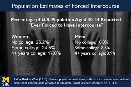
Women and men with four or more years of college reported lower rates of forced sexual intercourse. Women with fewer than four years of college education had 2.5 times higher odds of ever experiencing forced sexual intercourse then individuals with four or more years of college. For men with less than four years of college, the odds of ever experiencing forced sexual intercourse were 4 times higher compared to men with four or more years of college education. These findings generally held when adjusting for covariates associated with selection into college education. For both women and men, verbal pressure or abuse was the most frequently cited type of force experienced during the sexual assault.

The estimated rates of forced sexual intercourse highlight that sexual assault is a clear public health concern for both women and men, and in the decade between NSFG assessments there is no evidence of a decline in prevalence. It should also be noted that total sexual assault rates in the population are likely higher than reported here, because NSFG estimates are based on lifetime experiences and reflect only one subtype type of sexual assault. This underscores the need for more research to further characterize the full range of sexual assaults and associated consequences. Given that the majority of U.S. adults do not complete four or more years of college education, it is critical to expand intervention research to consider the unique contextual factors associated with individuals not attending college since these adults are at the highest risk for experiencing sexual assault.

William Axinn, Maura Bardos, Brady West (2018). General population estimates of the association between college experience and the odds of forced intercourse. Social Science Research, 70:131-143.

In a new article published in the Journal of Official Statistics, SRC Research Associate Professor James Wagner presents interesting collaborative research on interviewer travel with former Michigan Program in Survey Methodology (MPSM) graduate Kristen Olson, who is currently an Associate Professor of Sociology at the University of Nebraska-Lincoln. Clear gaps in knowledge exist in the survey methodology literature with respect to interviewer travel behaviors: we don’t really know what interviewers do daily, why they do what they do, or how these behaviors affect other important field outcomes. Interviewer travel is also a very important component of the overall field costs incurred by a face-to-face survey. Wagner and Olson specifically consider the relationships of interviewer travel patterns and behaviors with important field outcomes in two major face-to-face SRC surveys (the NSFG and the HRS), and they provide a compelling demonstration of the ability of paradata describing these patterns and behaviors to predict outcomes that are important to field operations.

More specifically, the authors consider the methodological approach of aggregating call record paradata from the NSFG and HRS to the interviewer-day level, and examine two important measures of interviewer travel that have important cost implications: the amount of distance traveled to different sampled area segments on each day, and the number of trips made to their assigned segments on each day. They also note various possible sources of error in these measures, which is an important point, and note that interviewer reports of distance traveled are highly correlated with what would be expected based on the locations of their homes.

Using cross-classified random effects models appropriate for each type of dependent variable, which account for crossed random effects of randomly selected interviewers and primary sampling units (PSUs), they initially consider various auxiliary predictors of these travel measures (including area features, such as size and an estimated difficulty of obtaining an interview measure from the Census Bureau, and interviewer characteristics, such as experience), to see what influences these travel decisions made by the interviewers in the two surveys. Next, they consider these travel outcomes as predictors of important survey outcomes, including contact attempts, contact rates, and response rates, controlling for the same auxiliary predictors. Separate rates were considered for both screening and main interviews, given the screening designs of the HRS and NSFG. I liked how the authors presented clear a priori expectations about the relationships of interest based on the very small amount of research that has currently been conducted (mainly based on simulation) in each case.

In their models, Wagner and Olson initially find evidence of substantial interviewer and area variance in terms of nearly all the outcomes, suggesting that interviewers vary substantially in terms of these travel behaviors and the field outcomes. But what might be the reasons for this variance? Considering their first question, they report that very few of the auxiliary predictors considered could predict total mileage traveled on a given day, in either survey. As a result, significant interviewer variance remains despite controlling for the various area and interviewer characteristics, which is an interesting finding. They did find some predictors of the number of segments visited: in the HRS, interviewers working in non-self-representing PSUs tended to visit more segments on each day, and more experienced interviewers tended to visit more segments as well. In both surveys, more segments were visited later in the field period. Considering their second question, they report that the number of segments visited on a given day had a positive relationship with the counts of screener and main attempts (for both surveys), as expected, for both surveys, and that the number of segments visited had a negative relationship with both contact rates and screening / main interview rates (again, for both surveys). These results held even when controlling for the number of miles traveled. However, the amount of distance traveled interestingly did not significantly predict any of these outcomes.

These findings have important practical implications for interviewer training, and the authors do a nice job of considering these implications for practice. Specifically, they strongly recommend careful monitoring of interviewer variance in the number of segments visited on each day, as an important tool for minimizing potential variance among interviewers in nonresponse bias. They also indicate that this monitoring should be used to initiate conversations with interviewers about their travel patterns and whether they could strive to be more efficient.

The authors have been working on this paper for a long time, and it made for clear and enjoyable reading. The paper makes a solid contribution to a growing literature on interviewer behaviors and the ability of survey paradata to describe these behaviors and their relationships with other important survey outcomes, and provides clear suggestions for practice for managers of field operations.

James Wagner and Kristen Olson (2018). An Analysis of Interviewer Travel and Field Outcomes in Two Field Surveys. Journal of Official Statistics, 34(1): 211-237.

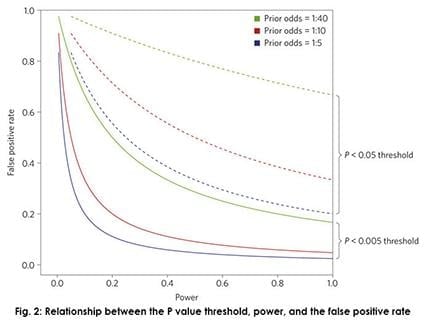
In a recent article, Redefine statistical significance, in Nature, one of the most highly-cited scientific publications worldwide, SRC Faculty Member Rod Little was part of a large team of co-authors that argues for the development of a new standard for statistical significance related to claims of new scientific discoveries (rather than reproduction of existing findings). In short, this team of co-authors argues that in many settings where p < 0.05 is the current standard for evidence of a new finding, including many of the social sciences, a threshold of p < 0.005 is more appropriate.

The authors begin by addressing the current crisis of lack of reproducibility in science, which could be due to misuse of certain indicators of statistical significance such as the p-value. The authors have a simple premise: ‘…statistical standards of evidence for claiming new discoveries in many fields of science are simply too low.’ They indicate that continued use of a ‘default’ standard of p < 0.05 likely results in too many false positive findings, and that such a threshold should now be referred to as ‘suggestive’ of an important finding.

The first major section of the article reviews the correct interpretation of p-values, and discusses the attractive properties of presenting evidence against a null hypothesis in terms of a Bayes factor and the estimated prior odds of an alternative hypothesis being true (relative to a specified null hypothesis). The authors speak to the relationship between the p-value and the Bayes factor in selected settings, presented compelling evidence of a choice of p < 0.05 corresponding to ‘weak’ or ‘very’ weak evidence in terms of Bayes factors. While nothing is said about how exactly Bayes factors might be computed in practice for those unfamiliar with the topic, the authors provide several relevant references on the topic.

The second major section of the article addresses the ‘Why 0.005?’ question. First, the authors again refer to the relationship between p-values and Bayes factors in selected hypothesis testing settings, and indicate that a choice of 0.005 would correspond to ‘substantial’ or ‘strong’ evidence in these settings, following conventional classifications of Bayes factors. Second, the authors show how this choice of a default threshold for significance would substantially reduce false positive rates, especially in studies with lower statistical power. Finally, the authors cite some recent studies that have demonstrated high potential gains in rates of reproducibility that would come from using this threshold.

I appreciated that the final ‘major’ section of the article presented reasonable objections to this choice of a new threshold, including increasing false negative rates. While this new threshold would require a necessary increase in the sample sizes of existing studies for a given choice of statistical power, the authors argue that there would be a benefit in terms of resources saved from studies that would no longer be conducted under false premises. Other objections include the fact that this procedure would not stop multiple testing or ‘p-hacking’ (a point with which the authors fully agree), thresholds for significance may vary for different scientific communities, and the fact that the use of p-values should cease all-together in favor of other measures of evidence such as effect sizes. The authors acknowledge that there is not yet widespread consensus that significance testing based on p­-values should be eliminated completely, and conclude by saying that journals can help with this transition to a new standard of evidence, given the shortcomings of the old (and indeed arbitrary) standard.

While I would have liked a little bit more information (or references) for practitioners about how Bayes factors should be computed in practice (again for those unfamiliar with the topic) and where estimates of prior odds in favor of an alternative hypothesis might come from in different fields, this short article still makes a compelling argument in favor of a new standard for statistical significance if various fields are going to continuing using p-values as an important measure of new scientific evidence.

This article was published in Nature:

Benjamin, Daniel J., Berger, James O., et al. (2017). Redefine statistical significance. Nature.